Solving the Vlasov-Poisson equation using Python
A plasma is a quasi-neutral gas of charged and neutral particles showing non-trivial collective behavior, distinct from other states of matter. The dynamics of plasma can be derived from the Boltzmann equation, where we can usually assume that we have a negligible amount of collisions. This leads us to the collisionless Boltzmann or Vlasov equation. In this tutorial, we want to simulate a simple one-dimensional plasma using the Vlasov equation and look at Landau damping and two kinetic instabilities. Since in one dimension we can’t have any magnetic fields, we actually solve the electrostatic Vlasov-Poisson equation.
Theory
If we want to simulate moving electrons, in principle we have to solve the full Maxwell system of equations, containing $E$ and $B$ fields. Since in the following we can safely assume the speed of the electrons $v$ to be much smaller than the speed of light $c$, i.e., $v\ll c$, we can neglect the contribution of the magnetic field and assume the effect of the electric field to be instantaneous. We know that the divergence of the electric field equals the charge density $$\nabla\cdot E=4\pi\rho$$ (in CGS units) and that in electrostatics the electric field can be derived from an electric potential $$E=-\nabla\phi.$$ Combined, we find Poissons equation for electrostatics $$\Delta\phi=4\pi\rho.$$
When simulating plasma, computational physicists usually use either the fluid discription of plasmas, called Magneto-Hydrodynmaics (MHD), or the semi-lagrangian Particle-In-Cell (PIC) method to sample the Vlasov equation. However, both approaches have their drawbacks. For example, the MHD theory is based on a few but fundamental assumptions which break down in certain, very interesting, regimes. PIC on the other hand does not have the limits on, e.g., resitivity, but needs a computationally very intensive amount of particles to generate solutions with a reasonable low amount of noise at a given space-time resolution.
The idea of simulating the Vlasov equation is to directly evolve the probability distribution function $f$ to find a charged particle in a given phase space region $\mathrm{d}x\mathrm{d}v$ at time $t$, i.e., the Vlasov equation is a 6+1 dimensional scalar function of position and velocity. However, since this is difficult to solve and we already learn a lot from simpler systems, we restrict the following discussion to the one-dimensional case.
For a plasma there are usually two distribution functions, one for ions and one for electrons. But since ion mass is typically much larger than the electron mass ($m_i\gg m_e$), electrons more much faster than ions. In such a case, we can assume a neutralizing ion background and only simulate electron dynamics. Using our assumptions, the Vlasov equation can be written as $$\frac{\mathrm{d}}{\mathrm{d}t} f(x, v,t) = 0,$$ where charge density is then simply the first moment of the Vlasov equation times the electron charge $q_e$ $$\rho(x,t)=q_e\int f(x,v,t) \mathrm{d}v$$
Taking the total time derivative of $f$ using the chain rule we find the plasma kinetic equation $$\frac{\mathrm{d}}{\mathrm{d}t} f=\frac{\partial f}{\partial t}+\frac{\partial x}{\partial t}\frac{\partial f}{\partial x}+\frac{\partial v}{\partial t}\frac{\partial f}{\partial v}=0$$
By identifying $\frac{\partial x}{\partial t}=v$ and $\frac{\partial v}{\partial t}=a$ and using the equation for electrostatic force $F_E=m_ea=q_e E$ we derived the 1D Vlasov-Poisson equation: $$\frac{\partial f}{\partial t}+v\frac{\partial f}{\partial x}+\frac{q_\alpha E}{m}\frac{\partial f}{\partial v}=0.$$ The form of this equation resembles a hyperbolic conservation law that can be computed numerically by employing standard techniques of fluid dynamics. For simplicity, in this tutorial we use the so-called upwind scheme.
Implementation
To run the simulation of the Vlasov equation on a computer we have to implement a finite difference scheme. As our programming language of choice is python, we have to take special care on performance. This obscures the readability of the code but makes python code run nearly as fast as C code. First we need to import our favorite libraries. Here we will mainly rely on numpy for computation and matplotlib for visualization.
1import matplotlib.pyplot as plt
2import numpy as np
3import scipy
4import tqdm
5from maxpy.style import dark_mode
6
7dark_mode(background="#191c1c")
8
9CMAP = plt.get_cmap("cmr.chroma")
Computing the electric field from a charge density using Fourier transforms
Fourier transform conventions
We define the Fourier transform and its inverse as
$$ f(\mathbf{k}) = \int_{\mathbb{R}^3} f(\mathbf{r}) e^{-i\mathbf{k}\cdot\mathbf{r}} , d^3 r $$
$$ f(\mathbf{r}) = \frac{1}{(2\pi)^3} \int_{\mathbb{R}^3} f(\mathbf{k}) e^{i\mathbf{k}\cdot\mathbf{r}} , d^3 k $$
Different conventions may redistribute factors of $2\pi$ without changing physical results.
Poisson’s equation in Fourier space
Using the correspondence
$$\nabla^2 \longrightarrow -k^2$$
Poisson’s equation becomes
$$-k^2 \phi(\mathbf{k}) = -4\pi\rho(\mathbf{k})$$
Solving for the potential gives
$$\phi(\mathbf{k}) = \frac{4\pi\rho(\mathbf{k})}{k^2}$$
This expression is valid for $k \neq 0$. The $k = 0$ mode corresponds to the total charge and requires separate treatment.
Electric field in Fourier space
Since $\mathbf{E} = -\nabla \phi$ and
$$\nabla \longrightarrow i\mathbf{k}$$
the electric field in Fourier space is
$$\mathbf{E}(\mathbf{k}) = -i\mathbf{k},\phi(\mathbf{k}) = -i\mathbf{k},\frac{4\pi\rho(\mathbf{k})}{k^2}$$
or equivalently
$$\mathbf{E}(\mathbf{k}) = i\frac{\mathbf{k}}{k^2}4\pi\rho(\mathbf{k})$$
Transforming back to real space
The real-space electric field is obtained by inverse Fourier transform:
$$\mathbf{E}(\mathbf{r}) = \frac{1}{(2\pi)^3} \int d^3 k ; \frac{i\mathbf{k}}{k^2}, \rho(\mathbf{k}), e^{i\mathbf{k}\cdot\mathbf{r}}$$
This expression is equivalent to Coulomb’s law:
$$\mathbf{E}(\mathbf{r}) = \int d^3 r’ ; \rho(\mathbf{r}’) \frac{\mathbf{r}-\mathbf{r}’}{|\mathbf{r}-\mathbf{r}’|^3}$$
Practical algorithm
Given $\rho(\mathbf{r})$:
- Compute $\rho(\mathbf{k})$ via a Fourier transform.
- Multiply by $\frac{i\mathbf{k}}{k^2}$ in Fourier space.
- Apply the inverse Fourier transform to obtain $\mathbf{E}(\mathbf{r})$.
Using spectral solvers for the Poisson equation is especially useful when we deal with periodic boundary conditions, since they are satisfied by definition. The real benefit, however, comes from the Fast Fourier Transform (FFT).
 1def solve_poisson_fft(rho, dx, nx):
 2    rho_k = np.fft.fft(rho)
 3    k_vals = 2 * np.pi * np.fft.fftfreq(nx, d=dx)
 4
 5    E_k = np.zeros_like(rho_k, dtype=complex)
 6    nonzero = k_vals != 0
 7    E_k[nonzero] = (1j / k_vals[nonzero]) * rho_k[nonzero]
 8
 9    E = np.real(np.fft.ifft(E_k))
10    return E
Upwind scheme
The upwind scheme is a finite difference or finite volume discretization method for hyperbolic partial differential equations. It accounts for the direction of information propagation.
1. Model problem
Consider the linear advection equation
$$\frac{\partial u}{\partial t} + a \frac{\partial u}{\partial x} = 0$$
where $a$ is a constant advection velocity. Characteristics propagate with speed $a$. The numerical flux is constructed using information from the upstream direction.
- If $a > 0$, information travels from left to right.
- If $a < 0$, information travels from right to left.
First order upwind discretization
Let $u_i^n \approx u(x_i, t^n)$ with spatial step $\Delta x$ and time step $\Delta t$.
Case $a > 0$
$$\frac{\partial u}{\partial x}\bigg|_{x_i} \approx \frac{u_i-u_{i-1}}{\Delta x}$$
The time update is
$$u_i^{n+1}=u_i^n-\frac{a \Delta t}{\Delta x}\left(u_i^n - u_{i-1}^n\right)$$
Case $a < 0$
$$\frac{\partial u}{\partial x}\bigg|_{x_i} \approx \frac{u_{i+1}^n - u_i^n}{\Delta x}$$
Conservative finite volume form
For a conservation law
$$\frac{\partial u}{\partial t} + \frac{\partial f(u)}{\partial x} = 0$$
the upwind numerical flux at interface $i+1/2$ is
$$F_{i+1/2} = \begin{cases} f(u_i), & f’(u) > 0 \\ f(u_{i+1}), & f’(u) < 0 \end{cases}$$
For linear advection $f(u) = a u$, this reduces to the previous formulas.
Stability condition
The upwind scheme is stable under the CFL condition
$$\frac{|a|\Delta t}{\Delta x} \le 1$$
With that, the method is first order accurate in space and in time. However, it introduces numerical diffusion proportional to $\Delta x$. The main advantage is that its unconditionally stable for hyperbolic problems and rather simple to implement. The disadvantage is low accuracy and smoothed gradients at shocks.
For our specific problem of the 1D Vlasov-Poisson equation, we have to split the advection in two steps, one to advance in velocity space and one to advance in position space, where we use different upwind conditions. We can achieve that in python by looping over all position and velocity cells and deciding case per case which sign to choose.
 1def _advance_velocity(f, dx, dt, nx, nv, v):
 2    for i in range(nx - 1):
 3        for j in range(nv - 1):
 4            if v[j] > 0:
 5                f[i, j] = f[i, j] - dt / dx * (f[i, j] * v[j] - f[i - 1, j] * v[j])
 6            else:
 7                f[i, j] = f[i, j] - dt / dx * (f[i + 1, j] * v[j] - f[i, j] * v[j])
 8    return f
 9
10
11def _advance_position(f, dv, dt, nx, nv, E):
12    for i in range(nx - 1):
13        for j in range(nv - 1):
14            if E[i] > 0:
15                f[i, j] = f[i, j] - dt / dv * (f[i, j] - f[i, j - 1]) * E[i]
16            else:
17                f[i, j] = f[i, j] - dt / dv * (f[i, j + 1] - f[i, j]) * E[i]
18    return f
However, this is very slow in python. We can significantly increase the speed by using numpy vectorization. This obscures the readability of the code, however results in a performance boost of approximately 100 times as fast as simple loops. The updates than look like the following functions
 1def advance_velocity(f, v, dx, dt, v_mask, v_mask_not):
 2    f[:, v_mask] = f[:, v_mask] - dt / dx * (f - np.roll(f, 1, axis=0))[:, v_mask] * v[v_mask]
 3    f[:, v_mask_not] = f[:, v_mask_not] - dt / dx * (np.roll(f, -1, axis=0) - f)[:, v_mask_not] * v[v_mask_not]
 4    return f
 5
 6
 7def advance_position(f, E, dv, dt, E_mask, E_mask_not):
 8    f[E_mask, :] = f[E_mask, :] - dt / dv * (f - np.roll(f, 1, axis=1))[E_mask, :] * E[E_mask][..., np.newaxis]
 9    f[E_mask_not, :] = (
10        f[E_mask_not, :] - dt / dv * ((np.roll(f, -1, axis=1) - f)[E_mask_not, :]) * E[E_mask_not][..., np.newaxis]
11    )
12    return f
Finally we can put everything together and implement the time loop. We store the results of every m’th time step into an array for later processing, such as creating a gif of the evolution.
1def get_initial_distribution(params):
2 # Allocate memory for the distribution function
3 f = np.zeros((params["nx"], params["nv"]))
4 x = np.linspace(0, params["L"], params["nx"], endpoint=False)
5 v = np.linspace(params["vmin"], params["vmax"], params["nv"])
6 dv = np.abs(v[1] - v[0]) # velocity step size
7 dx = np.abs(x[1] - x[0]) # spatial step size
8 dt = params["CFL"] * min(dx / params["vmax"], dv / 1.0) # assuming max|E| ~ 1
9
10 print("Simulation parameters:")
11 print(f" Spatial step size (dx): {dx}")
12 print(f" Velocity step size (dv): {dv}")
13 print(f" Time step size (dt): {dt}")
14
15 return f, x, v, dx, dv, dt
16
17
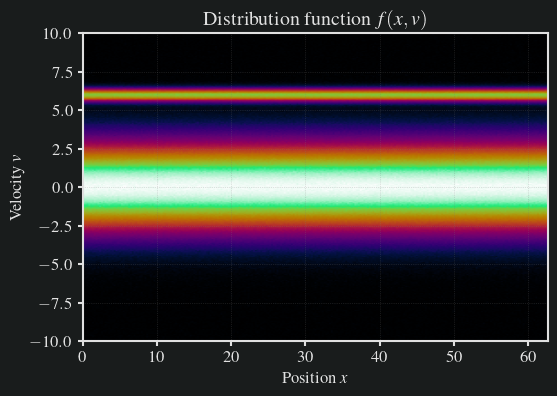
18def plot_distribution(f, x, v):
19 # plt.figure(figsize=(6, 4), dpi=100)
20 plt.imshow(f.T, cmap=CMAP, aspect="auto", origin="lower", extent=[x.min(), x.max(), v.min(), v.max()])
21 # plt.colorbar()
22 plt.title("Distribution function $f(x,v)$")
23 plt.xlabel("Position $x$")
24 plt.ylabel("Velocity $v$")
25 # plt.show()
26 return
27
28
29def run_simulation(f, x, v, dx, dv, dt, params):
30 # Allocate memory for the results
31 result = np.zeros((params["maxiter"] // params["save_interval"], params["nx"], params["nv"]))
32 E_k_hist = []
33
34 # Get masks for upwind schemes
35 v_mask = np.argwhere(v > 0)
36 v_mask_not = np.argwhere(v <= 0)
37
38 for it in tqdm.tqdm(range(params["maxiter"])):
39 # Advance velocity distribution
40 f_new = advance_velocity(f, v, dx, dt, v_mask, v_mask_not)
41
42 # Integrate f along velocity axis to get charge density
43 rho = params["q_e"] * np.trapezoid(f_new, dx=dv, axis=1)
44
45 # Add constant ion background
46 rho = rho - np.mean(rho)
47
48 # Solve Poisson equation
49 E = solve_poisson_fft(rho, dx, params["nx"])
50
51 # Get mask for upwind scheme
52 E_mask = np.argwhere(E > 0)
53 E_mask_not = np.argwhere(E <= 0)
54
55 # Advance position distribution
56 f_new = advance_position(f_new, E, dv, dt, E_mask, E_mask_not)
57
58 if params["export_mode"]:
59 # Solve Poisson with FFT
60 rho_k = np.fft.fft(rho)
61 k_vals = 2 * np.pi * np.fft.fftfreq(params["nx"], d=dx)
62
63 # Avoid division by zero at k=0
64 E_k = np.zeros_like(rho_k, dtype=complex)
65 nonzero = k_vals != 0
66 E_k[nonzero] = (1j / k_vals[nonzero]) * rho_k[nonzero]
67 E = np.real(np.fft.ifft(E_k))
68
69 # Save fundamental mode (k=±1 depending on domain length L)
70 # If domain length is L=2π/k0, then fundamental mode index is 1
71 E1 = E_k[1] / params["nx"]
72 E_k_hist.append(E1)
73
74 # Save every mth step
75 if it % params["save_interval"] == 0:
76 result[it // params["save_interval"]] = f.copy()
77 if params["plot"]:
78 plot_distribution(f, x, v)
79 plt.savefig(f"/home/max/Temp/{params['name']}_{it:05d}.png")
80 return result, E_k_hist
Kinetic instabilities in collisionless plasmas
In collisionless plasmas, wave propagation and stability are described by the Vlasov equation coupled to Poisson’s equation. Landau damping, the two stream instability, and the bump on tail instability arise from resonant wave particle interactions.
Linearizing around a homogeneous equilibrium $f_0(v)$ leads to the electrostatic dispersion relation
$$1 + \frac{1}{k^2 \varepsilon_0}\sum_s \frac{q_s^2}{m_s}\int \frac{\partial f_{0s}/\partial v}{v - \omega/k} , dv= 0$$
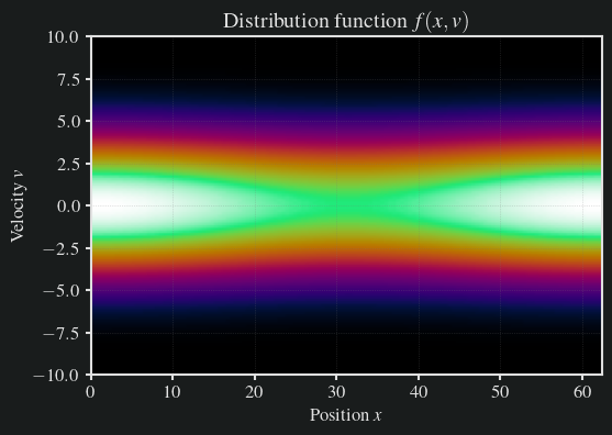
Landau damping
Landau damping occurs when the equilibrium distribution function $f_0(v)$ is monotonic decreasing. The imaginary part of the wave frequency is obtained by evaluating the dispersion relation using the Landau contour, yielding
$$\gamma =\operatorname{Im}(\omega)=-\frac{\pi}{2}\frac{\omega_p^2}{k}\left.\frac{\partial f_0}{\partial v}\right|_{v = \omega_r/k}$$
where $\omega_p$ is the plasma frequency and $\omega_r$ is the real part of the wave frequency. For $\partial f_0 / \partial v < 0$, the damping rate $\gamma$ is negative, corresponding to exponential decay of the wave amplitude.
 1params = {
 2    "nx": 128 + 1,  # Number of spatial positions
 3    "nv": 128 + 1,  # Number of velocity values
 4    "vmin": -10,  # Minimal possible velocity
 5    "vmax": 10,  # Maximal possible velocity
 6    "q_e": -1,  # Electron charge
 7    "n_particles": 1,  # Initial particle number
 8    "k": 0.1,  # wave number of perturbation
 9    "L": 2 * np.pi / 0.1,  # domain length for k
10    "CFL": 0.5,  # CFL number
11    "maxiter": 4000,  # Maximum number of iterations
12    "plot": True,  # Whether to plot intermediate results
13    "save_interval": 100,  # Save every mth step
14    "export_mode": True,  # Whether to export mode data
15    "save_path": "/home/max/Temp",  # Path to save output files
16    "name": "landau_damping",  # Simulation name
17}
18
19
20def maxwellian(v, vbeam, vth):
21    return np.exp(-0.5 * ((v - vbeam) / vth) ** 2) / (np.sqrt(2 * np.pi) * vth)
22
23
24# Get initial distribution and simulation parameters
25f, x, v, dx, dv, dt = get_initial_distribution(params)
26
27# Maxwellian
28vth = 3.0
29f0 = maxwellian(v, 0.0, vth)
30
31# Small perturbation
32alpha = 1e-1
33f = np.zeros((params["nx"], params["nv"]))
34for i in range(params["nx"]):
35    f[i, :] = f0 * (1 + alpha * np.cos(params["k"] * x[i]))
36
37# Normalize the distribution
38f = f / f.sum()
39
40plot_distribution(f, x, v)
Simulation parameters:
  Spatial step size (dx): 0.4870686284635338
  Velocity step size (dv): 0.15625
  Time step size (dt): 0.02435343142317669
1result, E_k_hist = run_simulation(f, x, v, dx, dv, dt, params)
  0%|          | 0/4000 [00:00<?, ?it/s]

100%|██████████| 4000/4000 [00:38<00:00, 102.75it/s]
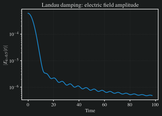
 1E_k_hist = np.array(E_k_hist)
 2t = np.arange(len(E_k_hist)) * dt
 3
 4# Amplitude of first Fourier mode
 5amp = np.abs(E_k_hist)
 6
 7plt.plot(t, amp)
 8plt.yscale("log")
 9plt.xlabel("Time")
10plt.ylabel(r"$|E_{k=0.5}(t)|$")
11plt.title("Landau damping: electric field amplitude")
12plt.show()
 1# find peaks
 2peaks, _ = scipy.signal.find_peaks(amp)
 3plt.plot(t[peaks], amp[peaks], "x")
 4plt.yscale("log")
 5plt.xscale("log")
 6plt.xlabel("Time")
 7plt.ylabel(r"$|E_k(t)|$")
 8plt.grid(which="both", linestyle="--", linewidth=0.5)
 9plt.show()
10
11# get slope
12fit_range = (t > 0.5) & (t < 30)
13slope, intercept, *_ = scipy.stats.linregress(t[peaks], np.log(amp[peaks]))
14
15print(f"Numerical damping rate gamma = {slope:.4f}")
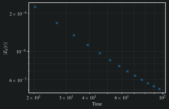
Numerical damping rate gamma = -0.0184
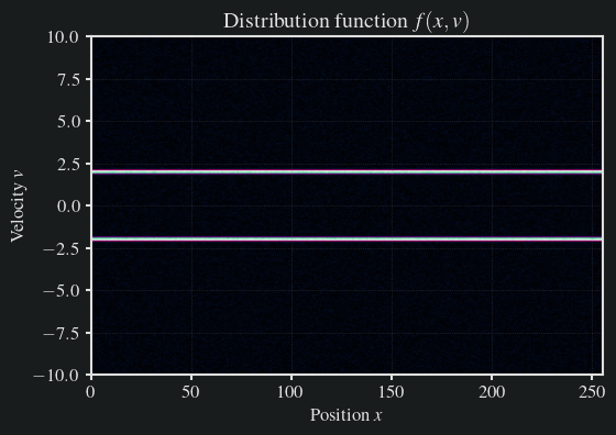
Two stream instability
The two stream instability arises when the equilibrium distribution consists of two drifting populations. A simple cold plasma model uses
$$f_0(v) =\frac{n_0}{2}\left[\delta(v - v_0) + \delta(v + v_0)\right]$$
The resulting dispersion relation is
$$1 - \frac{\omega_p^2}{(\omega - k v_0)^2}- \frac{\omega_p^2}{(\omega + k v_0)^2}= 0$$
For sufficiently large drift velocity $v_0$, this equation admits solutions with $\operatorname{Im}(\omega) > 0$, indicating exponential growth of electric field perturbations.
 1params = {
 2    "nx": 256 + 1,
 3    "nv": 256 + 1,
 4    "vmin": -10,
 5    "vmax": 10,
 6    "q_e": -1000,
 7    "n_particles": 1,
 8    "k": 0.1,
 9    "L": 256,
10    "CFL": 0.5,
11    "maxiter": 4000,
12    "plot": True,
13    "save_interval": 100,
14    "export_mode": True,
15    "save_path": "/home/max/Temp",
16    "name": "two_stream_instability",
17}
18
19# Get initial distribution and simulation parameters
20f, x, v, dx, dv, dt = get_initial_distribution(params)
21
22vth = 0.01 * params["vmax"]  # Thermal velocity
23vbeam = 0.2 * params["vmax"]  # Beam velocity
24
25# Initial distribution for two-stream instability
26for i in range(params["nv"]):
27    f[:, i] = np.exp(-((v[i] - vbeam) ** 2) / vth**2) + np.exp(-((v[i] + vbeam) ** 2) / vth**2)
28
29# Add noise
30f += np.random.normal(0, 0.01, f.shape)
31
32# Normalize the distribution
33f = f / f.sum()
34
35# Plot initial distribution
36plot_distribution(f, x, v)
Simulation parameters:
  Spatial step size (dx): 0.9961089494163424
  Velocity step size (dv): 0.078125
  Time step size (dt): 0.0390625
1result, E_k_hist = run_simulation(f, x, v, dx, dv, dt, params)
  0%|          | 0/4000 [00:00<?, ?it/s]

100%|██████████| 4000/4000 [00:43<00:00, 91.53it/s]
Bump on tail instability
The bump on tail instability occurs when the distribution function has a local maximum at high velocity, so that
$$\left.\frac{\partial f_0}{\partial v}\right|_{v = \omega/k}> 0$$
The growth rate follows the same expression as Landau damping but with opposite sign,
$$\gamma =-\frac{\pi}{2}\frac{\omega_p^2}{k}\left.\frac{\partial f_0}{\partial v}\right|_{v = \omega_r/k}$$
A positive slope at the resonant velocity leads to $\gamma > 0$, corresponding to wave amplification.
 1params = {
 2    "nx": 256 + 1,
 3    "nv": 256 + 1,
 4    "vmin": -10,
 5    "vmax": 10,
 6    "q_e": -1,
 7    "n_particles": 1,
 8    "k": 0.1,
 9    "L": 2 * np.pi / 0.1,
10    "CFL": 0.5,
11    "maxiter": 4000,
12    "plot": True,
13    "save_interval": 100,
14    "export_mode": True,
15    "save_path": "/home/max/Temp",
16    "name": "bump_on_tail",
17}
18
19# Get initial distribution and simulation parameters
20f, x, v, dx, dv, dt = get_initial_distribution(params)
21
22vth = 0.2 * params["vmax"]  # Thermal velocity
23vbeam = 0.6 * params["vmax"]  # Beam velocity
24
25alpha_b = 0.1
26eps = 1e-4
27
28fM = lambda v, u, vt: np.exp(-((v - u) ** 2) / (2 * vt**2)) / (np.sqrt(2 * np.pi) * vt)
29
30f0v = (1 - alpha_b) * fM(v, 0, vth) + alpha_b * fM(v, vbeam, 0.3)
31
32f = np.zeros((params["nx"], params["nv"]))
33for i in range(params["nx"]):
34    f[i, :] = f0v * (1 + eps * np.cos(10 * x[i]))
35
36f += np.random.normal(0, 0.001, f.shape)
37
38f /= np.sum(f[0, :]) * dv
39
40# Plot initial distribution
41plot_distribution(f, x, v)
Simulation parameters:
  Spatial step size (dx): 0.24448191856729906
  Velocity step size (dv): 0.078125
  Time step size (dt): 0.012224095928364953
1result, E_k_hist = run_simulation(f, x, v, dx, dv, dt, params)
  0%|          | 0/4000 [00:00<?, ?it/s]

100%|██████████| 4000/4000 [00:43<00:00, 92.12it/s]
Summary
All three phenomena are described by the same linearized Vlasov dispersion relation. Landau damping corresponds to negative slope of the distribution function at resonance, while the two stream and bump on tail instabilities arise from nonmonotonic velocity distributions that provide free energy for wave growth.
The jupyter notebook of this tutorial can be downloaded here
>> Home