In this tutorial we want to simulate a stream of electrons in the Pierce Diode in one dimension using the electrostatic Vlasov-Poisson Equation. When simulating such a scenario, usually computational plasma physicists use either the fluid discription of plasmas, called Magneto Hydrodynmaics (MHD), or the semi-lagrangian Particle-In-Cell method to simulate the Vlasov equation. However, both approaches have their drawbacks. For example, the MHD theory is based on a few but fundamental assumptions which break down in certain, very interesting, regimes. PIC on the other hand does not have the limits on e.g.resitivity but needs a computationally very intensive amount of particles to generate solutions with a reasonable low amount of noise at a given space-time resolution.
1
2
3
4
5
6
import tqdm
import cmasher
import numpy as np
import matplotlib.pyplot as plt
plt.style.use("dark")
plt.style.use({'figure.facecolor': '#111213'})
The idea of simulating the Vlasov equation is to directly evolve the distribution function, which is a 6+1 dimensional scalar function of position and velocity. Formally it can be written as
\[\frac{\mathrm{d}}{\mathrm{d}t} f(\vec{x},\vec{v},t) = 0\]Usually there are two distribution functions, one for ions and one for electrons. But as we only want to simulate electron dynamics we can omit the ion part here. Taking the total time derivative using the chain rule we find the plasma kinetic equation
\[\frac{\mathrm{d}}{\mathrm{d}t} f=\frac{\partial f}{\partial t}+\frac{\partial x}{\partial t}\frac{\partial f}{\partial x}+\frac{\partial v}{\partial t}\frac{\partial f}{\partial v}=0\]By identifying $\frac{\partial x}{\partial t}=v$ and $\frac{\partial v}{\partial t}=a$ and using the equation for electrostatic force $F_E=m_ea=q_e E$ we derived the 1D Vlasov-Poisson equation:
\[\frac{\partial f}{\partial t}+v\frac{\partial f}{\partial x}+\frac{q_\alpha E}{m}\frac{\partial f}{\partial v}=0\]This is generally a hyperbolic conservation law and can be computed numerically by employing standard techniques of solving partial differential equation like the Lax-Wendroff scheme or similar. In this tutorial we use the very simple upwind scheme.
The final missing ingredient to solve the Vlasov equation is the electric field. The problem is that if we want to simulate moving electrons in principle we have to solve the full Maxwell system of equations, containing E and B fields. In our case however we can neglegt the contribution of the magnetic field and calculate the electric field simply from the Poission equation using the charge density distribution $\rho$. First we know that the divergence of the electric field equals the charge density
\[\nabla\cdot E=4\pi\rho\]The charge density can simply be found as the first moment of the Vlasov equation, hence
\[\rho(x,t)=q_e\int f(x,v,t) \mathrm{d}v\]Implementation
To run the simulation of the Vlasov equation on a computer we have to implement a finite difference scheme. As our programming language of choice is python, we have to take special care on performance. This obscures the readability of the code but makes python code run nearly as fast as C code.
We start by implementing gradients and laplacians in matrix form. The gradient can be approximated by central differences
\[\frac{\partial f(x)}{\partial x}\approx\frac{f(x+h)-f(x-h)}{2h}\]The corresponding matrix using periodic boundary condition is thus
\[\begin{pmatrix}0 & 1/2 & 0 & ... & -1/2\\ -1/2 & 0 & 1/2 & ... & 0\\ \cdots &&&& \\ 1/2 &0&0& ... & 0\end{pmatrix}\]1
2
3
4
5
6
7
8
9
def gradient(n):
matrix = np.diag(np.ones(n)*0)
matrix += np.diag(np.ones(n-1)*0.5, 1)
matrix += np.diag(np.ones(n-1)*-0.5, -1)
matrix[0,-1] = -0.5
matrix[-1,0] = 0.5
return matrix
print(gradient(6))
1
2
3
4
5
6
[[ 0.   0.5  0.   0.   0.  -0.5]
 [-0.5  0.   0.5  0.   0.   0. ]
 [ 0.  -0.5  0.   0.5  0.   0. ]
 [ 0.   0.  -0.5  0.   0.5  0. ]
 [ 0.   0.   0.  -0.5  0.   0.5]
 [ 0.5  0.   0.   0.  -0.5  0. ]]
The Laplacian $\Delta$ in 1D can be approximated by central differences as well, yielding
\[\Delta f(x)=\frac{\partial^2 f(x)}{\partial x^2}\approx\frac{f(x+h)-2f(x)+f(x-h)}{h^2}\]with corresponding matrix form
\[\begin{pmatrix}-2 & 1 & 0 & ... & 1\\ 1 & -2 & 1 & ... & 0\\ \cdots &&&& \\ 1 &0&0& ... & 2\end{pmatrix}\]1
2
3
4
5
6
7
8
9
def laplace(n):
matrix = np.diag(np.ones(n)*-2)
matrix += np.diag(np.ones(n-1), 1)
matrix += np.diag(np.ones(n-1), -1)
matrix[0,-1] = 1
matrix[-1,0] = 1
return matrix
print(laplace(6))
1
2
3
4
5
6
[[-2.  1.  0.  0.  0.  1.]
 [ 1. -2.  1.  0.  0.  0.]
 [ 0.  1. -2.  1.  0.  0.]
 [ 0.  0.  1. -2.  1.  0.]
 [ 0.  0.  0.  1. -2.  1.]
 [ 1.  0.  0.  0.  1. -2.]]
Solving the Poisson Equation
To solve the Poisson equation given a density distribution we will use a simple iterative approach. For this we implement the Jacobi algorithm to solve linear systems of equations. We can evalute as much Jacobi steps as we like to solve the system to a satisfying degree, either by an break criterium or by a fixed number of steps.
1
2
3
4
5
6
7
8
9
10
11
12
13
14
15
def jacobi(A,b,N=25,x=None):
    """Solves the equation Ax=b via the Jacobi iterative method."""
    # Create an initial guess if needed
    if x is None:
        x = np.zeros(len(A[0]))

    # Create a vector of the diagonal elements of A
    # and subtract them from A
    D = np.diag(A)
    R = A - np.diagflat(D)

    # Iterate for N times
    for i in range(N):
        x = (b - np.dot(R,x)) / D
    return x
The Simulation loop
To evolve the Vlasov equation we iterate over discrete timesteps. The main simulation loop will do the following:
- Advance distribution function in velocity direction
- Calculate charge density from distribution function
- Approximate electric potential from charge density via Jacobi iterations
- Calculate electric field by taking the gradient of the potential
- Advance distribution function in spatial direction with electric field
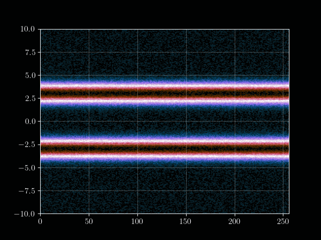
We start by defining some simulation constants and construct our initial distribution. The initial position ditribution is a simple uniform distribution and the velocity distribution as an maxwellian (or simply gaussian).
1
2
3
4
5
6
7
8
9
10
11
12
13
14
15
16
17
18
19
20
21
22
23
24
25
26
27
28
29
30
31
32
33
34
35
36
37
38
nx = 256 # Number of spatial positions
nv = 256 # Number of velocity values
maxiter = 30000 # Maximal number of iterations
maxiter_jacobi = 30 # Maximal number of Jacobi steps
dt = 0.001 # Time step size
dx = 0.1 # Spatial step size
vmin = -10 # Minimal possible velocity
vmax = 10 # Maximal possible velocity
vth = 0.1*vmax  # Thermal velocity
vbeam = 0.8*nv # Beam velocity
q_e = -1 # Electron charge
n_particles = 2# Initial particle number

# Allocate memory for the
f = np.zeros((nx, nv))
v = np.linspace(vmin, vmax, nv)
dv = np.abs(v[1] - v[0]) # velocity step size

# Construct gradient and laplace matrices
gradient_matrix = gradient(nx)
laplace_matrix = laplace(nx)

# Construct plasma in thermal equilibrium
for i in range(nv):
    #f[:, i] = np.exp(-(v[i]-3)**2/vth**2) + np.exp(-(v[i]+3)**2/vth**2)
    f[:, i] = n_particles * np.exp(-(v[i])**2/vth**2)

f += np.random.random(f.shape)*0.1*n_particles

# Get index for beam velocity
idx = int(vbeam)

# Plot initial distribution
plt.imshow(f.T, cmap=plt.get_cmap("cmr.lavender"), aspect="auto", origin="lower", extent=[0, nx, vmin, vmax])
plt.colorbar()
plt.title("Initial distribution function $f(x,v,t=0)$")
plt.xlabel("Position $x$")
plt.ylabel("Velocity $v$")
In principle the only thing left is implementing the time steps. This can be done with two python loops using the upwind scheme. This means we use forward differences when the advection velocity is smaller than zero and backward differences when the velocity is bigger than zero
1
2
3
4
5
6
7
8
9
10
11
12
13
14
15
16
17
def advance_velocity(f):
    for i in range(nx-1):
        for j in range(nv-1):
            if v[j] > 0:
                f[i,j] = f[i,j] - dt/dx*(f[i,j]*v[j] - f[i-1,j]*v[j])
            else:
                f[i,j] = f[i,j] - dt/dx*(f[i+1,j]*v[j] - f[i,j]*v[j])
    return f

def advance_position(f, E):
    for i in range(nx-1):
        for j in range(nv-1):
            if E[i] > 0:
                f[i,j] = f[i,j] - dt/dv*(f[i,j] - f[i,j-1])*E[i]
            else:
                f[i,j] = f[i,j] - dt/dv*(f[i,j+1] - f[i,j])*E[i]
    return f
However, this is very slow in python. We can significantly increase the speed by using numpy vectorization. This obscures the readability of the code, however results in a performance boost of approximately 100 times as fast as simple loops. The updates than look like the following functions
1
2
3
4
5
6
7
8
9
def advance_velocity(f, v_mask):
    f[:,v_mask] = f[:,v_mask] - dt/dx*(f[:,v_mask]*v[v_mask] - np.roll(f, 1, axis=0)[:,v_mask]*v[v_mask])
    f[:,~v_mask] = f[:,~v_mask] - dt/dx*(np.roll(f, -1, axis=0)[:,~v_mask]*v[~v_mask] - f[:,~v_mask]*v[~v_mask])
    return f

def advance_position(f, E, E_mask):
    f[E_mask,:] -= dt/dv*((f[E_mask,:].T*E[E_mask]).T - (np.roll(f, 1, axis=1)[E_mask,:].T*E[E_mask]).T)
    f[~E_mask,:] = f[~E_mask,:] - dt/dv*((np.roll(f, -1, axis=1)[~E_mask,:] - f[~E_mask,:]).T*E[~E_mask]).T
    return f
The masks can easily be computed by using numpy masking, however the mask for the electric field has to be computed in each step, while the velocity can be computed in advance.
1
v_mask = np.argwhere(v > 0)
Finally we can put everything together and implement the time loop. We store the results of every m’th time step into an array for later processing, such as creating a gif of the evolution.
1
2
3
4
5
6
7
8
9
10
11
12
13
14
15
16
17
18
19
20
21
22
23
24
25
26
27
28
29
30
31
32
33
34
35
36
37
38
39
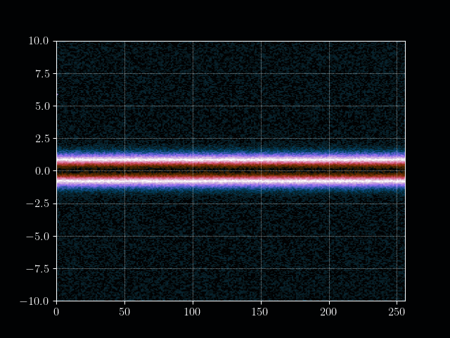
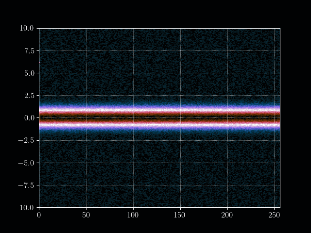
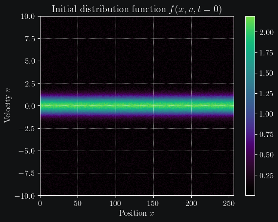
# Plot ever mth step
m = 100
# Allocate memory for the results
result = np.zeros((maxiter//m, nx, nv))
plot = False
for it in tqdm.tqdm(range(maxiter)):
# Inject electron beam into simulation
f[0,idx + int(np.random.normal(0,7))] = 1
# Advance velocity distribution
f = advance_velocity(f, v_mask)
# Integrate number density along velocity density to get charge density
rho = q_e*np.sum(f, axis=1)
# Add constant ion background
rho = rho + np.mean(rho)
# Calculate potential via some Jacobi steps
phi = jacobi(laplace_matrix, rho, N=maxiter_jacobi)
# Calculate electric field
E = - gradient_matrix@phi
# Get mask for upwind scheme
E_mask = E > 0
# Advance position distribution
f = advance_position(f, E, E_mask)
# Save every mth step
if it%m==0:
result[it//m] = f.copy()
if plot:
plt.imshow(f.T, cmap="inferno",aspect="auto", origin="lower", extent=[0, nx, vmin, vmax])
plt.show()
1
100%|██████████| 30000/30000 [00:32<00:00, 915.47it/s]